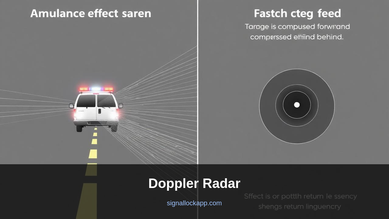
The Doppler effect in 30 seconds
When a wave source moves toward you, the waves arrive more often — higher frequency. When it moves away, lower frequency. You hear it with sirens. Radar sees it with reflected pulses. If the transmitter emits at 10.000 GHz and the echo returns at 10.0001 GHz, the target is closing at roughly 3 metres per second.
Why Doppler is hard to fake
Chaff, decoys and most stealth tricks can hide a radar return's size but not its velocity. A moving target produces a Doppler shift; a stationary metal strip does not. This is why pulse-Doppler radar dominates modern fighter intercept — it filters out ground clutter that has zero Doppler shift and shows only the things actually moving.
Weather radar in colour
A NEXRAD weather radar fires 1000+ pulses a second in a slowly rotating beam. Each raindrop reflects a tiny return. The system computes the Doppler shift per range cell and colours the map by it: green for raindrops moving toward the antenna, red for raindrops moving away. The boundary between green and red, with strong shifts on both sides, is the signature of a rotating storm — a mesocyclone that may produce a tornado.
Police radar guns
A handheld police radar is a continuous-wave Doppler device. It fires a microwave beam at your car, listens for the reflection, and measures the frequency shift. At 24 GHz, every 1 m/s of closing speed produces about 160 Hz of shift. A small DSP chip converts the shift directly to km/h.
The Pulse-Doppler processing gap
A critical technical hurdle in early Doppler systems was the 'blind speed' phenomenon. Because pulse-Doppler radar samples the target's position at discrete intervals, a target moving at a specific velocity can travel exactly one or more wavelengths between pulses. To the processor, the phase shift appears to be zero, making a fast-moving jet look like a stationary mountain. Engineers solved this by employing staggered pulse repetition frequencies (PRF). By varying the timing between pulses, the system ensures that a target invisible at one frequency becomes detectable at the next, allowing for continuous tracking across all relevant speed brackets.
To process these shifts, modern hardware uses Fast Fourier Transforms (FFT) to convert time-domain signals into frequency-domain data. This allows the radar to separate a single return into multiple 'bins' based on velocity. In a complex environment, this technology allows a radar to simultaneously track a slow-moving rain shower, a high-speed aircraft, and the stationary ground beneath them. Without this digital separation, the massive 'clutter' from the earth's surface would overwhelm the receiver, rendering it impossible to detect any low-flying objects or subtle wind shears near airports.
The transition from CW to Pulse
The earliest Doppler experiments relied on Continuous Wave (CW) radar, which emits a constant stream of energy. While CW is excellent at measuring precise velocity—as seen in basic handheld police guns—it suffers from a major flaw: it cannot measure distance. Because there is no 'start' or 'stop' to the signal, the time of flight cannot be calculated. This limited early 1940s research until the development of coherent pulse oscillators allowed engineers to combine the ranging capabilities of traditional radar with the velocity-sensing power of the Doppler shift.
This evolution culminated in the 1950s with the AN/APG-66 and similar airborne units, which allowed 'look-down/shoot-down' capability. Before this, an interceptor looking down toward the earth would see only a blinding glare of reflected energy from the ground. By applying Doppler filters, the radar ignores the static ground and highlights only the moving aircraft. This shift in signal processing fundamentally changed aerial warfare, ensuring that low-altitude flight was no longer a reliable way to hide from radar surveillance.
The Unambiguous Range Limit
In pulse-Doppler systems, engineers face a classic trade-off known as the Doppler dilemma. To measure high velocities accurately, the radar must send pulses at a high pulse repetition frequency (PRF). However, if a subsequent pulse is sent before the echo from the first pulse returns, the system cannot determine which pulse corresponds to which reflection. This creates 'range ambiguities' where a target appears much closer than it actually is. Finding the balance between measuring the speed of a jet and correctly identifying its distance requires sophisticated PRF switching, a technique perfected in the late 1970s for the F-15’s APG-63 radar.
The mathematical constraint is rigid: the product of the maximum unambiguous range and the maximum unambiguous velocity is limited by the speed of light. If you increase the range to see further, you must decrease the PRF, which lowers the maximum speed you can detect without the frequency 'aliasing'—a phenomenon where a fast-moving object appears to be moving slowly or even in the opposite direction. Modern digital signal processors (DSPs) solve this by using staggered PRFs and multiple pulse widths, effectively 'de-aliasing' the signal in real-time to provide a clear picture of both distance and velocity simultaneously.
Christian Doppler's 1842 Discovery
While we associate the effect with sophisticated electronics, Christian Doppler first proposed the theory in 1842 to explain the colors of binary stars. To prove it for sound, scientist C.H.D. Buys Ballot conducted a famous experiment in 1845 using a steam locomotive. He hired professional trumpeters to play a constant note while riding on an open flatcar passing through Utrecht at 64 kilometers per hour. Observers on the ground, gifted with perfect pitch, confirmed the pitch rose as the train approached and dropped as it passed. It took another century for the MIT Radiation Laboratory to apply these acoustic observations to microwave frequencies.
The shift from theoretical physics to practical radar occurred during World War II, but the technology truly matured in the 1960s with the development of the Coherent Oscillator (COHO). Before this, radars were 'non-coherent,' meaning they couldn't remember the exact phase of the transmitted pulse, making frequency shift detection nearly impossible. The COHO provided a stable reference, allowing the receiver to compare the return signal's phase to the original. This breakthrough transformed radar from a simple detection tool into a precision instrument capable of isolating a single moving vehicle against the background of a massive mountain range.