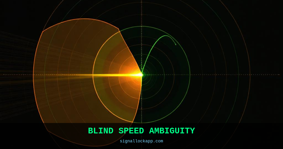
The blind speed formula
In an MTI or pulse-Doppler radar, a target whose radial velocity causes exactly one full phase rotation between pulses (360°) has the same phase as stationary clutter. It cancels perfectly. The blind speeds are v = nλ·PRF/2, where n is any integer. A 3 GHz radar with 1,000 Hz PRF has blind speeds at 50 m/s, 100 m/s, 150 m/s — a jet at exactly 180 knots (93 m/s) would vanish.
Staggered PRF
The fix is simple in theory: change the PRF so the blind speeds shift. A two-stagger PRF (e.g. 1,000 Hz and 1,200 Hz) makes a target blind at one PRF visible at the other. Military radars use multiple stagger patterns, sometimes changing every pulse. Digital processing then unscrambles the pattern and recovers the true velocity.
Range ambiguity
High PRF for velocity means short unambiguous range: R_unambiguous = c/(2·PRF). At 100 kHz PRF, the maximum unambiguous range is 1.5 km. An echo arriving after 2 µs could be a target at 300 km on the current pulse, or a target at 150 km from the previous pulse — ambiguous. Multiple PRFs and phase coding resolve which is which.
Modern solutions
Digital signal processing and variable PRF have essentially solved blind speeds and range ambiguity in modern systems. But the physics remains: a pulsed radar is a sampled system, and sampling creates aliasing. Understanding these ambiguities is still core to radar engineering education — and to interpreting why a target sometimes 'jumps' on screen.
The Pulse-Doppler Dilemma
The trade-off between range and velocity measurement is often called the radar dilemma. In high-PRF pulse-Doppler systems, frequently used in fighter aircraft search modes, the priority is eliminating ground clutter and detecting high-speed targets. However, this high pulse frequency creates extreme range ambiguity. The radar might see a target clearly, but because the pulse interval is so short, the echo could belong to any of several preceding pulses. To solve this, radars employ M-out-of-N algorithms where the system transmits several different PRFs in rapid succession. Only a target at a specific true range will produce detections that align across all the different timing ‘bins’ used in the pulse sequence.
Historically, this limitation defined the development of the AN/AWG-9 radar for the F-14 Tomcat in the 1960s. Engineers had to balance the need to detect bombers at 160 kilometers with the requirement to track incoming missiles at Mach 3. By utilizing a variable PRF strategy, they managed to push the first blind speed outside the envelope of expected aerial targets while relying on complex digital timing circuits to resolve the range. This illustrates that radar design is rarely about finding a perfect frequency, but rather about managing the mathematical inevitabilities of Nyquist-Shannon sampling theorems in a physical three-dimensional space.
Second-Time-Around Echoes
A common misconception is that energy from beyond the unambiguous range simply disappears. In reality, exceptionally large targets—like mountains or tankers—can produce ‘second-time-around’ or even ‘third-time-around’ echoes. These signals return after the radar has already sent its next pulse, causing the processor to plot the target much closer than it actually is. In early analog systems, these phantom targets were indistinguishable from real ones. Modern coherent radars use pulse-to-pulse phase shifting, or 'phase coding,' to label each transmitted pulse with a unique signature. If the returning echo's phase does not match the most recent transmission, the system identifies it as an ambiguous range return and can either filter it or calculate its true distance.
During the Cold War, early warning radar stations in the Arctic frequently dealt with anomalous propagation where atmospheric ducting carried signals far beyond the horizon. Technicians would see 'ghost' targets moving at impossible speeds across the scope. These were actually ships or landmasses hundreds of miles away, appearing within the radar's first range gate due to high PRF settings. The transition from simple MTI filters to sophisticated Doppler Filter Banks allowed for better separation of these signals. By comparing the signal-to-noise ratios and the phase stability across multiple bursts, modern processors can effectively 'de-alias' the data, ensuring that the operator sees a single, coherent tactical picture rather than a screen filled with overlapping echoes.
The Butterfly Effect in MTI Display
In the analog era of Moving Target Indication (MTI), technicians identified blind speeds through a visual phenomenon known as the 'butterfly effect' on Plan Position Indicators (PPI). When a target's radial velocity approached a multiple of the pulse repetition frequency, the return pulse would appear to shimmer or fluctuate in intensity before vanishing entirely. This occurred because the phase difference between the target signal and the reference oscillator was shifting slowly, causing the subtractor circuit to oscillate between constructive and destructive interference. It served as a critical early warning for radar operators that a fast-moving threat was approaching a blind velocity interval.
To mitigate this without the luxury of modern digital signal processors, early systems like the AN/FPS-6 height-finder used acoustic delay lines filled with mercury to store the previous pulse's return. By matching the delay exactly to the PRF interval, the system could subtract the stored pulse from the incoming one. However, temperature fluctuations in the mercury would change the speed of sound within the delay line, inadvertently shifting the blind speeds and creating 'clutter leakage.' This technical limitation forced constant calibration and was one of the primary drivers for the transition to solid-state quartz delay lines and eventually digital memory buffers.
Eclipse and the Zero-Doppler Notch
A common misconception is that blind speeds only occur at high multiples of the PRF. In reality, the most significant blind speed is zero—the 'clutter notch.' Because ground clutter (trees, buildings, terrain) has a radial velocity of zero, radar filters must suppress all signals near the zero-frequency bin. This creates a detection gap for targets flying tangentially to the radar. If a pilot performing a 'beaming' maneuver keeps their aircraft perpendicular to the radar beam, their radial velocity drops to zero, and they disappear into the clutter notch. Modern Pulse-Doppler systems use adaptive notch widths to minimize this window while still suppressing environmental noise.
Another specific challenge is 'eclipsing' in high-PRF radars, which differs from standard range ambiguity. Eclipsing occurs when a target return arrives exactly when the radar is transmitting its next pulse. Since the receiver is blanked during transmission to protect it from high-power damage, any echo returning during that window is lost. This creates 'blind zones' in range that are distinct from blind speeds in velocity. Engineers solve this by employing PRF jittering, ensuring that a target eclipsed at one frequency will likely be visible at the next, effectively 'filling' the range holes through statistical frequency diversity.